Human Activity Analysis
Research Problems
Human activity is an inherently dynamic process that can be understood beyond doubt when the temporal evolution is also taken into account. For example, an image depicting a certain pose of the human figure can be confused with any kind of gait e.g. walking, running or even speed walking or walking with a limp but a video, even over a very small time frame, can immediately allude to the viewer the exact nature of the gait. The dynamics of a particular action are a very crucial tool in identifying and understanding the action. The goal of this research is to better understand the dynamics behind the human activity process as captured in videos and to use these to perform recognition of the action in any given video.
Feature Selection
Selecting the right features for the representation of human motion dynamics is the first step towards developing a recognition paradigm. We cannot just use intensity or color trajectories as they are not representative of the true motion. In the past, researchers have used motion capture data, however accurately extracting limbs and joints from a video without using stick-up markers is difficult. Moreover, there is always the question whether the representation should be unique to the whole person i.e. global, or whether a collection of local representations such as a parts-based approach is better. Global motion models allow for the construction of a spatially compact and temporally consistent formulation. However the drawback is that these models break down when there is a large amount of occlusion of the subject, in which case parts-based or local approaches are applicable. Local models however do not take into account of the dynamics of the scene. Since our goal is to explicitly model the dynamics of human motion, we propose a global model.
Assuming that there is only one person moving in the scene and the background is stationary, we first compute the optical flow for each frame of the entire video. We quantize the optical flow as shown in figure 2. Each optical flow vector is binned according to its principal angle with the horizontal. The contribution to each bin is wiehted by the magnitude of the optical flow vector. This gives us a scale and fronto-parallel direction invariant feature, a Histogram of Oriented Optical Flow (HOOF) in each frame. The time series of such HOOF represents the motion in the scene.
System Identification
Since HOOF features are histograms and do not lie in a Euclidean space, we cannot model HOOF time series as Linear Dynamical Systems. Instead, we model the temporal evolution of HOOF features using a linear-state non-linear dynamical system using kernels on the space of histograms,
where Φ is an implicit map of a kernel on the space of histograms. Some of the metrics that can be used with the kernel are the Bhattacharrya distance, Χ2 distance, the Histogram Intersection kernel, and the Minimum Distance Pairwise Assignment. Using Kernel PCA, we identify the parameters ymean, x0, A, B and the covariance of the noise processes v and w, as well as the kernel principal components that represent the C function.
Classification of Human Activities
Once the system parameters have been identified, we need to define a measure of affinity between two given Non Linear Dynamical Systems. A family of such measures between two Linear Dynamical Systems were introduced by Vishwanathan et. al. as the family of Binet Cauchy kernels. One of these kernels, called the trace kernel between two ARMA model can be evaluated as:


Since we cannot use LDS to model HOOF trajectories, we need an affinity measure that is applicable to the non-linear dynamical systems. We propose the Binet-Cauchy kernels for non-linear dynamical systems as:


Once an affinity measure has been defined between two non-linear dynamical systems, we use k-Nearest Neighbors (k-NN) Classification. Also to perform more sophisticated classification, we can use kernel SVMs with the previously defined kernels.

Results
We perform Leave-one-out classification using the Binet-Cauchy kernels for non-linear dynamical systems on the HOOF trajectories for the Weizmann human action dataset. This dataset contains 10 actions performed by 9 persons each for a total of 90 videos. For each video, HOOF feature time series were extracted and the corresponding system parameters were identified. For the test video, the Binet-Cauchy kernel for NLDS was computed with all the training videos and the label of the nearest one was assigned to the test video. The results were averaged over all the videos using a leave-one-out scheme. The confusion matrix for the classification results is shown below.s


Lip Articulation Analysis
Research Problems
We examine the dynamics of lips when people utter their name, as part of an identification phrase, or utter a digit from 0 to 9. We want to understand the dynamics behind the speech process as captured in videos and want to use these to do recognition of the person or recognition of the spoken digit.
Feature Selection
Selecting the right features for the representation of lip dynamics is the first step towards developing a recognition paradigm. We cannot use intensity or color trajectories as they are not representative of the true lip dynamics. We also cannot use motion capture data as that is not suitable for a possible biometrics application. We hence use a 3-stage processing system consisting of the following steps:
(a) Remove the natural head motion during the speaking act
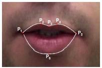
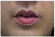
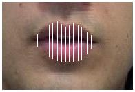
(b) Extract outer lip contours to collect six key-points on the lips and track these points throughout the video
(c) Interpolate from these six points to a total of 32 equi-distant points on the lip contours and record two types of features:
   1. Landmarks - The coordinates of these points,
   2. Distances - The distance between corresponding landmarks on the upper lip and the lower lip.

Lip contours Landmark features Distance features
System Identification
We model the temporal evolution of different lip features using the Linear Dynamical Systems Framework. More specifically, a sequence of feature trajectories is assumed to be a realization from a second-order stationary stochastic process and hence it can be modeled with a state space model:

To find the parameters for the Linear Dynamical System M = (x0, A, B, C, R) we consider the use of two popular Linear System Identification methods, namely:
1. N4SID
2. PCA-based suboptimal ID
Classification of Lip Articulation
Once the system parameters have been identified using any of the above mentioned methods, we need to define a measure of affinity between two given Linear Dynamical Systems. Over the past few years, a number of metrics have been proposed on the space of linear dynamical systems. A number of distances are based on the notion of subspace angles between two systems. These subspace angles are precisely the angles between the infinite observability matrices of the two systems. Since the infinite observability matrices cannot be found in a practical situation, we can estimate the subspace angles indirectly through the solution of a generalized eigen-value problem that translates to finding the solution of a Lyapunov equation. Once the subspace angles, {θi}2ni=1, have been found, a number of distances can be defined as:
Finsler distance
Martin distance
Frobenius distance

Another method for defining a measure of affinity between two LDS is through a kernel. The Martin Kernel, defined as:
Martin kernel

comes directly from the associated Martin Distance and is immediately computable from the subspace angles. Chan and Vasconcelos proposed another metric based on the Kullback-Leibler Divergence between the probability distributions of the outputs of the dynamical systems:


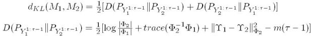
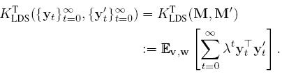
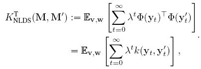
Vishwanathan et. al. introduced the family of Binet Cauchy kernels for the analysis of dynamical systems. One of these kernels, called the trace kernel between two ARMA model can be evaluated as:


Once an affinity metric has been defined between two linear dynamical systems, we use k-Nearest Neighbors (k-NN) Classification in the case of distances or k-Furthest Neighbors (k-FN) Classification for kernels. Also to perform more sophisticated classification, we use kernel SVMs with the previously defined kernels.

Results
We perform a large number of experiments, based on both the scenarios, namely 'Name' and 'Digit' using both the Landmarks features and the Distances features. To evaluate the performance of the different lip features, identification methods, distances and kernels for LDSs, and classification methods, we performed classification of the data sets G4, G8, and G12 (G12 is a group of 12 people who's lip motions were investigated. G4 is a smaller group of the first 4 people of these 12 people and G8 consists of the first 8 people) using leave-one-out classification. The following figure shows the group make up:


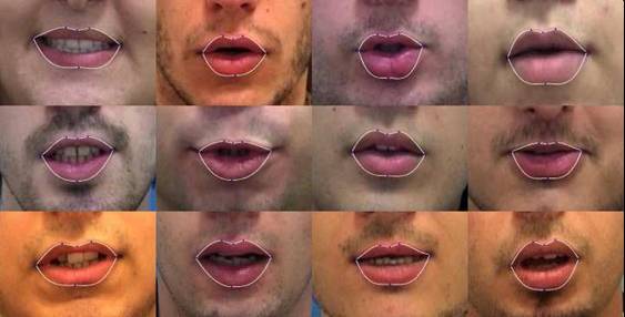
Groups - First row of the figure shows G4, the first 2 rows make up G8 and all the figures together represent G12.

The following table shows the classification errors of all groups in the name and digit scenarios for landmark trajectories, L, using the PCA-based identification method, and using both 1-NN classification with 5 different distances and SVM classification with 3 different kernels.


  1-NN SVM
PCA-L dFdMdfdKLkT kMkKLkT
G4 38131030 1700
G8 6341252333 451533
G12 6349343639 471740
Name scenario
  1-NN SVM
PCA-L dFdMdfdKLkT kMkKLkT
G4 4328151328 401010
G8 5546303445 411336
G12 6348334351 642043
Digit scenario
Publications
[1]
R. Chaudhry, A. Ravichandran, G. Hager and R. Vidal.
IEEE Conference on Computer Vision and Pattern Recognition, June 2009.
[2]
R. Chaudhry and R. Vidal.
Department of Computer Science, Johns Hopkins University, Technical Report 09-01.
[3]
E. Cetingul, R. Chaudhry and R. Vidal.
International Workshop on Dynamical Vision, October 2007.
Acknowledgments
This work was partially supported by the grants: NSF CAREER 0447739, NSF CDI-1 0941463, and ARL Robotics-CTA 80014MC.